🗺️ Biogeographic Domains and Bocaina de Minas

🌍 Overview

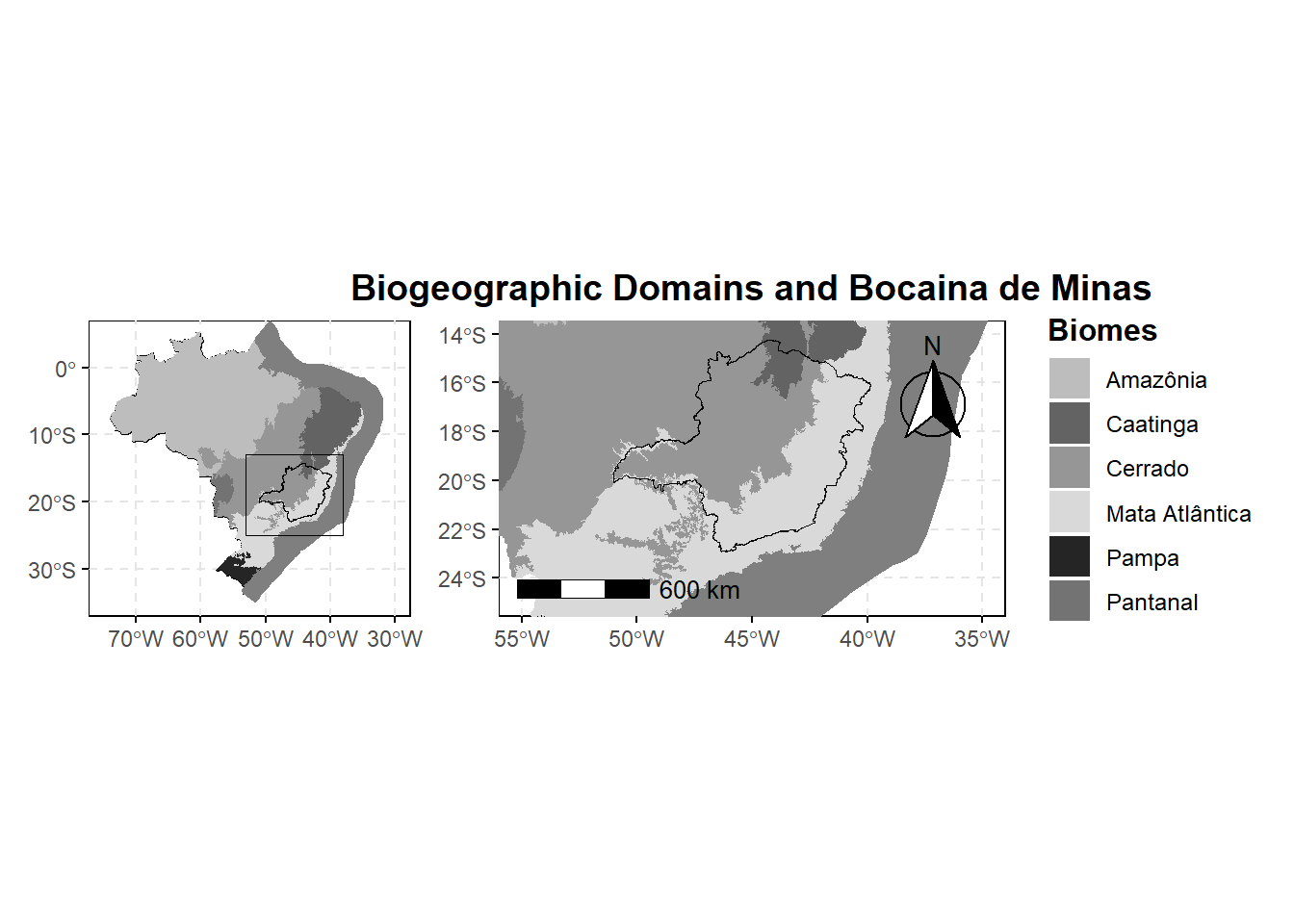
This post walks through the creation of a detailed map highlighting Brazil’s biogeographic domains with a focus on the state of Minas Gerais and a specific location, Bocaina de Minas. The workflow leverages R’s geospatial packages including sf, geobr, and ggplot2, and demonstrates how to combine multiple maps using patchwork.

📦 Loading Required Libraries

We start by loading the essential R packages:

library(sf)
library(tidyverse)
library(rnaturalearth)
library(rnaturalearthdata)
library(geobr)
library(ggspatial)
library(patchwork)

📥 Loading and Filtering Spatial Data

biomes <- read_biomes()

Using year/date 2019

states <- read_state()

Using year/date 2010

mg_state <- states %>% filter(abbrev_state == "MG")

📍 Geocoding Bocaina de Minas

bocaina <- data.frame(
  name = "Bocaina de Minas",
  lon = -44.5242,
  lat = -22.1694
) %>%
  st_as_sf(coords = c("lon", "lat"), crs = 4326)

🔲 Creating a Study Area Rectangle

rectangle <- st_as_sf(
  st_sfc(
    st_polygon(list(rbind(
      c(-53, -25), c(-38, -25),
      c(-38, -13), c(-53, -13),
      c(-53, -25)
    )))
  ),
  crs = 4326
)

🗺️ Map A: Brazil with Biomes and Rectangle

# Map A: Brazil with biomes, MG state, and study area rectangle
map_a <- ggplot() +
  # Plot all Brazilian states
  geom_sf(data = states, fill = "gray90", color = "black", size = 0.3) +
  
  # Overlay biomes with specific gray scale fill colors
  geom_sf(data = biomes, aes(fill = name_biome), color = NA) +
  
  # Highlight Minas Gerais with a bold border
  geom_sf(data = mg_state, fill = NA, color = "black", size = 0.9) +
  
  # Draw rectangle for study area
  geom_sf(data = rectangle, fill = NA, color = "black", size = 1.2) +
  
  # Set manual fill colors for biomes (greyscale palette)
  scale_fill_manual(
    values = c(
      "Amazônia" = "#bdbdbd",
      "Caatinga" = "#636363",
      "Cerrado" = "#969696",
      "Mata Atlântica" = "#d9d9d9",
      "Pampa" = "#252525",
      "Pantanal" = "#737373"
    )
  ) +
  
  # Set map coordinates to zoom out over all Brazil
  coord_sf(xlim = c(-75, -30), ylim = c(-35, 5)) +
  
  # Use minimal theme
  theme_minimal() +
  
  # Customize plot appearance
  theme(
    legend.position = "none",
    panel.background = element_rect(fill = NA, color = "black", linewidth = 0.5),
    panel.grid.minor = element_blank(),
    panel.grid.major = element_line(color = "grey90", linewidth = 0.5, linetype = "dashed"),
    axis.ticks = element_line(color = "black"),
    legend.title = element_text(face = "bold")
  )

map_a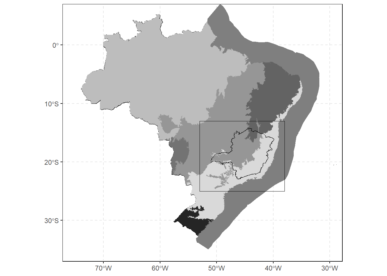

🗺️ Map B: Zoomed Biomes and Labelled Region

# Map B: Focused view with cartographic elements
map_b <- ggplot() +
  # Plot biomes
  geom_sf(data = biomes, aes(fill = name_biome), color = NA) +
  
  # Highlight MG state
  geom_sf(data = mg_state, fill = NA, color = "black", size = 0.9) +
  
  # Optional: highlight Bocaina de Minas as a red point
  # geom_sf(data = bocaina, color = "red", size = 3) +
  
  # Focus the map view over southeastern Brazil
  coord_sf(xlim = c(-55, -35), ylim = c(-25, -14)) +
  
  # Set biome color palette again
  scale_fill_manual(
    name = "Biomes",
    values = c(
      "Amazônia" = "#bdbdbd",
      "Caatinga" = "#636363",
      "Cerrado" = "#969696",
      "Mata Atlântica" = "#d9d9d9",
      "Pampa" = "#252525",
      "Pantanal" = "#737373"
    )
  ) +
  
  # Add north arrow and scale bar
  annotation_north_arrow(location = "tr", which_north = "true",
                         style = north_arrow_fancy_orienteering()) +
  annotation_scale(location = "bl", width_hint = 0.3,
                   text_cex = 0.8, line_width = 0.7) +
  
  # Apply clean theme
  theme_minimal() +
  
  # Customize plot appearance
  theme(
    panel.background = element_rect(fill = NA, color = "black", linewidth = 0.5),
    plot.title = element_text(hjust = 0.5, size = 14, face = "bold"),
    legend.title = element_text(size = 12, face = "bold"),
    legend.text = element_text(size = 9),
    legend.position = "right",
    panel.grid.minor = element_blank(),
    panel.grid.major = element_line(color = "grey90", linewidth = 0.4, linetype = "dashed"),
    axis.ticks = element_line(color = "black")
  ) +
  
  # Title for the plot
  labs(title = "Biogeographic Domains and Bocaina de Minas")

map_b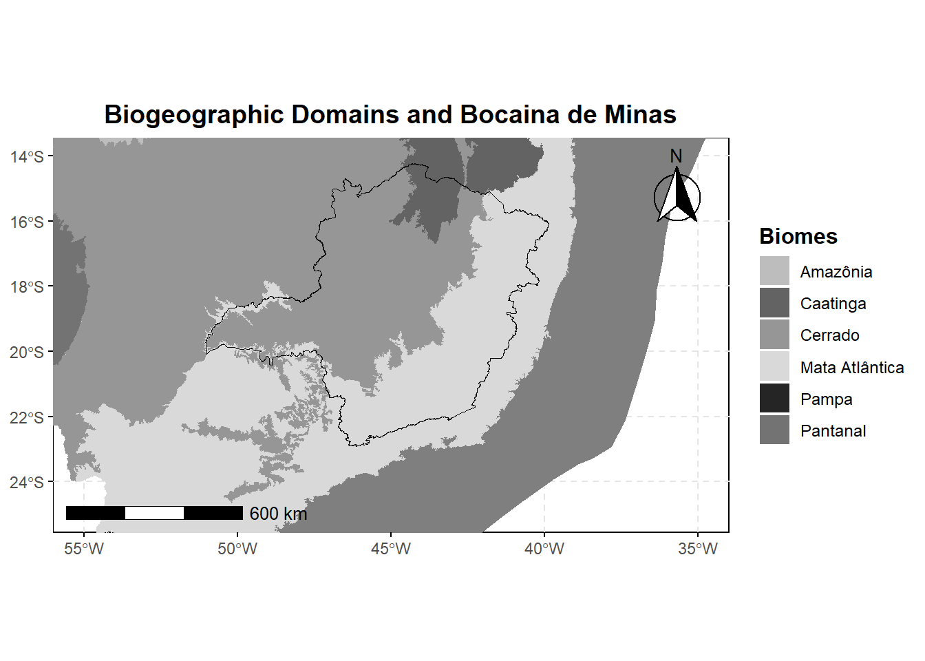

🧩 Combining the Two Maps

biomes_brazil = map_a + map_b + plot_layout(ncol = 2)

📊 Final Visualization

biomes_brazil